
SLAM Core
SLAMLab estimates the 6DoF trajectory of a lidar sensor while simultaneously constructing a map of the environment. The trajectory and map are incrementally updated with each new scan.
General concept
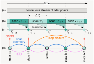
Section titled “General concept”A lidar sensor provides a continuous stream of individually timestamped points (a). For real-time processing, this stream is split into chunks called scans, e.g. a single ROS 2 message (b). In case of a rotating lidar, a single scan typically corresponds to one full 360° rotation with a duration of 50-100ms. Each scan is deskewed using either a constant velocity model or IMU-based inertial odometry (c). The SLAM pipeline then estimates the current optimal trajectory using a factor graph that incorporates lidar odometry, IMU preintegration, GNSS, and loop closure constraints (d).
Processing pipeline
Section titled “Processing pipeline”Processing is divided into three parallel threads: a main thread that applies a processing pipeline to each new scan, a loop closure detection thread, and a visualization thread.
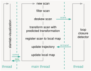
The main thread processes each scan in six steps:
- Filter scan — Remove unnecessary points using various filters, reducing the scan to ~20k–30k points.
- Deskew scan — Compensate for sensor motion during the scan. Uses either a constant velocity model or IMU-based inertial odometry.
- Transform scan with predicted pose — Predict the current pose and transform the deskewed scan into the map frame.
- Register scan to local map — Match planes extracted from the current scan against planes in the local map using point-to-plane ICP.
- Update trajectory — Re-estimate the full trajectory via factor graph optimization.
- Update local map — Merge planes from current scan into the local map.
At the end of a SLAM run, artifacts are saved to disk.